
There's always a push for better products. It's possible to put AI into an 8-bit microcontroller. It won't be like the large language models we're used to, but we can put neural networks into very low-cost products. We'll break down an example of how to put a neural network into a whole series of parts, how to optimize it, and what real world performance looks like (flash & performance).
So instead of being able to chat with you, this will make decisions. It will decide how long the microwave should run before the food is cooked. Or it will decide what kind of sound it's hearing. Or it could decide if your vacuum cleaner needs to be repaired. These devices don't need to make decisions constantly, instead they only need to do it once in a while (e.g. say we only need to check the sound once every second). Since we don't need to make decisions constantly, we get the advantage of being able to slowly make a decision -- as opposed to detecting instantly.
High End Options
There's a lot of well developed projects for running neural networks on higher end microcontrollers. If you have a lot of extra resources (say an extra 100kB of flash and RAM) -- you should look at LiteRT (TensorFlow Lite) or some of the similar frameworks. These classes of solutions originally targeted mobile applications and are great for high end microcontrollers. Everything we talk about in here applies to using LiteRT or any of the other frameworks.
Running on Cheap MCUs
Most people believe you can't run a neural network on an 8-bit MCU like a PIC16, a PIC18, an 8-bit AVR (like the Arduino Uno), or even the 16-bit MSP430. So we put the same neural network on all of them (plus a bunch of other parts for comparison). This series talks about how we did it and practical results.
So I've done this in the field several times, but I can't share the details of customer products. Instead, I've made up a simple detection problem where we are sampling a signal to identify what kind of signal it is. So our microcontroller is going to sample 32 times, and from those samples it makes a decision about which signal it saw in those samples.
The real magic of this is that we can apply this logic on parts with far less computational capability by delaying calculations and decisions until it's done. Below we'll show different decision times based upon different microcontrollers with identical algorithms and neural networks.
The Data
So we start with the signals we are going to detect.
Four kinds of signal: a sine, a square wave, a chirp (a sine whose frequency sweeps up across the window), and band-limited noise. Each example is 32 consecutive 8-bit ADC readings. To keep it honest, every window gets its own frequency, phase, amplitude, DC offset, and added noise, so the classes overlap and nothing is trivially separable. The top row below is the textbook shape of each; the bottom row is what the network actually sees.
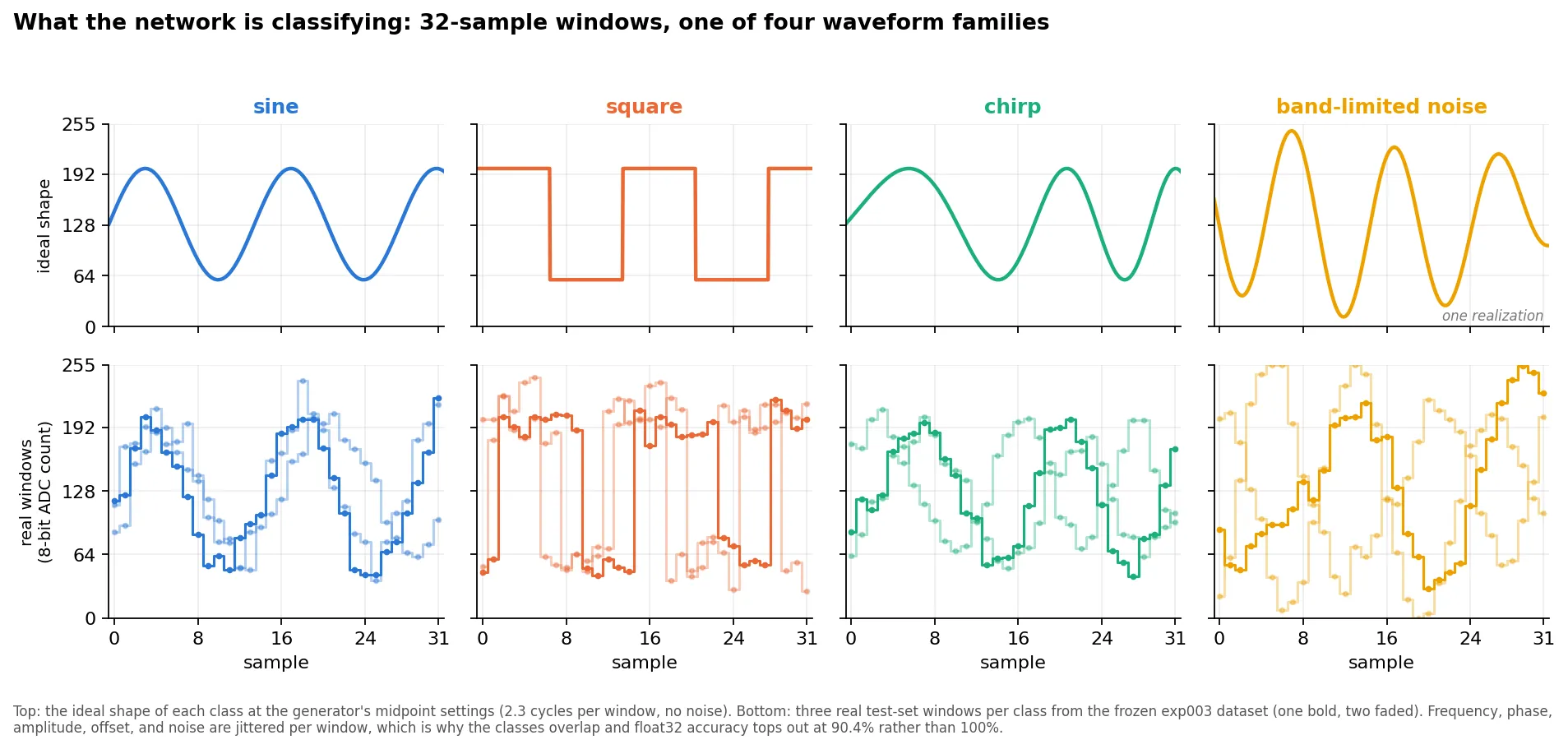
The dataset is synthetic: 4,096 training signals, 512 for validation, 512 held out for test, balanced across the four classes. The whole thing is 160 KB. We'll never need this data on the microcontroller, only on our PC where we do our training.
The network
A small multilayer perceptron: 32 inputs, hidden layers of 32, 16, and 8 with ReLU, four outputs. Whichever output is largest is the answer. That's 1,756 parameters and 1,696 multiply-adds per decision. Stored as 32-bit floats the weights are about 7 KB. (The experiment also has two shallower networks; I'll bring those in next time. This note sticks with the deepest one.)
If you haven't worked with neural networks before, here's the whole thing in two pictures. First the structure. The 32 samples go in on the left, and every line carries one number to a neuron in the next layer. This is a real window from the test set going through the real trained network.
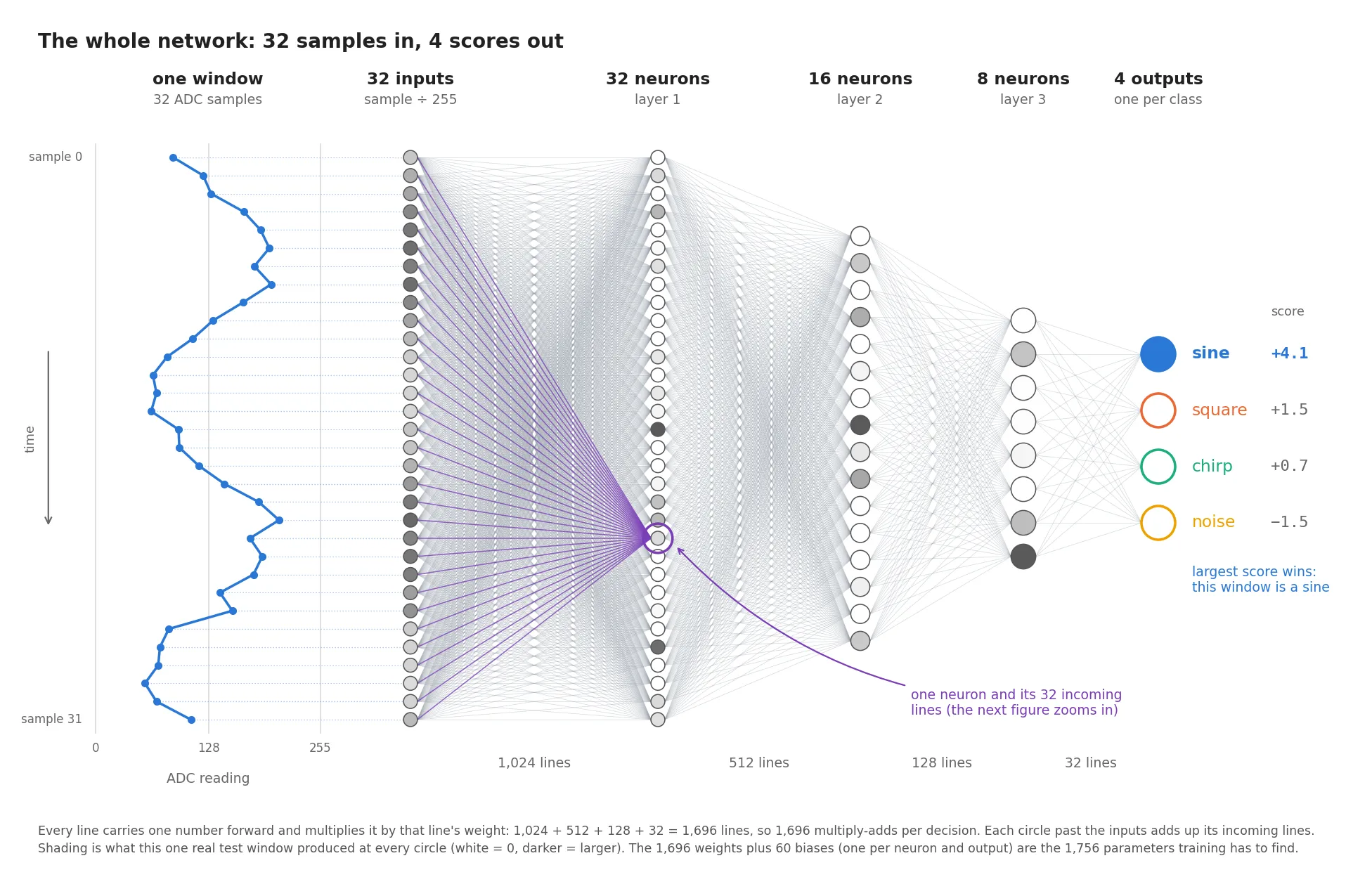
So each neuron performs several multiplies and accumulates (MACs). It multiplies each input by that line's weight, adds them all up, and adds one more constant (the bias). If the result is negative, it outputs zero instead. That last step is the ReLU. A ReLU is a fancy name for setting negative values to zero. Here's the neuron from the picture above with its actual numbers.
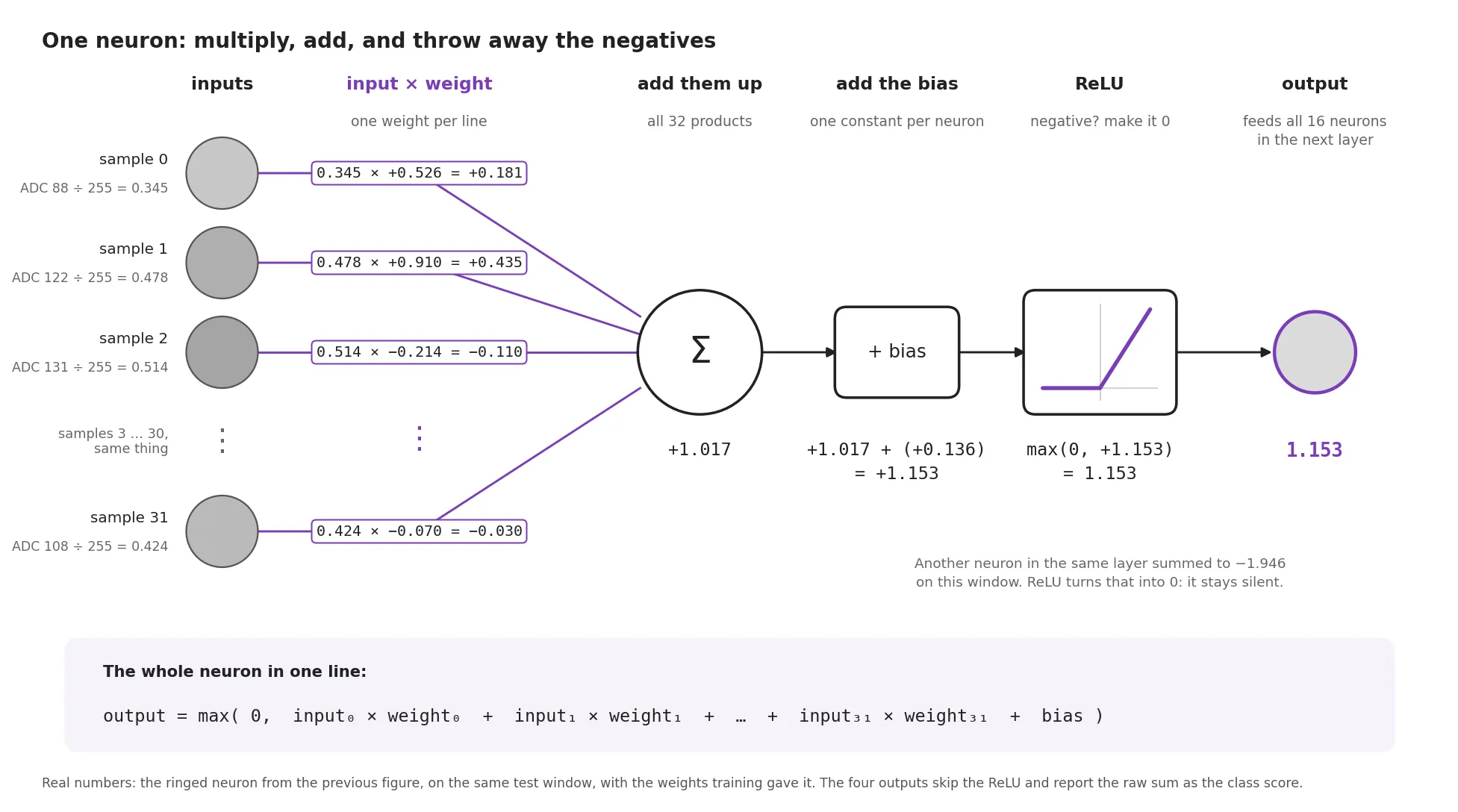
That's all the math there is. The firmware is that same loop run once for every circle in the first picture. Training is the search for the 1,756 weights and biases that make the right output come out largest.
The training method we used is deliberately boring: Adam, learning rate 0.01, every one of the 4,096 training windows in every step, 80 steps, in plain NumPy. It runs in under a second on a laptop and it's deterministic, which matters because the boards later have to prove they're running these exact weights. Final score: 90.9% on the training windows, 90.4% on the 512 test windows it never saw.
Watching it learn
Here's the part most people find fascinating: you can watch the model learn while it trains. Each square below is one class of training data, the same color as its waveform above: 1,024 windows laid out 32 by 32. Each cell is colored by what the network called that window. A solid square means every window of that class was classified correctly. The animation steps through all 80 training epochs.
A few things worth watching for:
- Epoch 0 is almost all orange. With random weights the network calls nearly everything a square (87% of the windows). Accuracy starts at 24%, which makes sense because we have four types of results and an equal amount of them in our training data.
- Square and noise come apart first. By epoch 3 the noise square is already turning yellow. Square has flat tops and noise has none, so that's the easiest line to draw.
- Sine and chirp take until epoch 15 to 20. They're both smooth, both roughly the same frequency, and the only difference is whether the frequency drifts across the window. Right around epoch 20 you can see the square column get worse for a while (45% at epoch 20) as the network re-draws its boundaries to make room for sine.
- The last 40 epochs are cleanup. 77% at epoch 40, 86% at 60, 91% at 80. The cells that never flip are the genuinely ambiguous windows: a low-amplitude square buried in noise, a chirp whose sweep happened to be small.
The mistakes it ends with are the ones you'd expect. On the test set, 7 sines were called squares and 8 squares were called sines. 9 noise windows were called squares. 6 sines were called chirps and 7 chirps were called sines. Nothing was wildly wrong; the network is confused exactly where the data is confusing.
Running it on 16 boards
Now the firmware. Same weights, written out as C arrays, with a straightforward float32 inference loop: multiply, add, ReLU, repeat. No vendor NN library, no SIMD intrinsics, nothing a PIC16 compiler couldn't swallow. So there's room for performance improvements on all of these -- but this is a consistent simple baseline.
I ran all of this on my benchmark fleet: 16 build targets on 15 physical boards, six ISA families (Cortex-M0+ through M7, RISC-V, Xtensa, AVR, MSP430, and Microchip PIC16/PIC18/PIC24/dsPIC33A). Every board gets flashed with real firmware and timed over serial, same harness and calibration rules as the arithmetic and FIR filter experiments. Each board also runs 64 of the test windows and reports a checksum of its outputs, which has to match the host bit for bit. So when I say a board "runs the network," I mean it produced the same answers as the Python model.
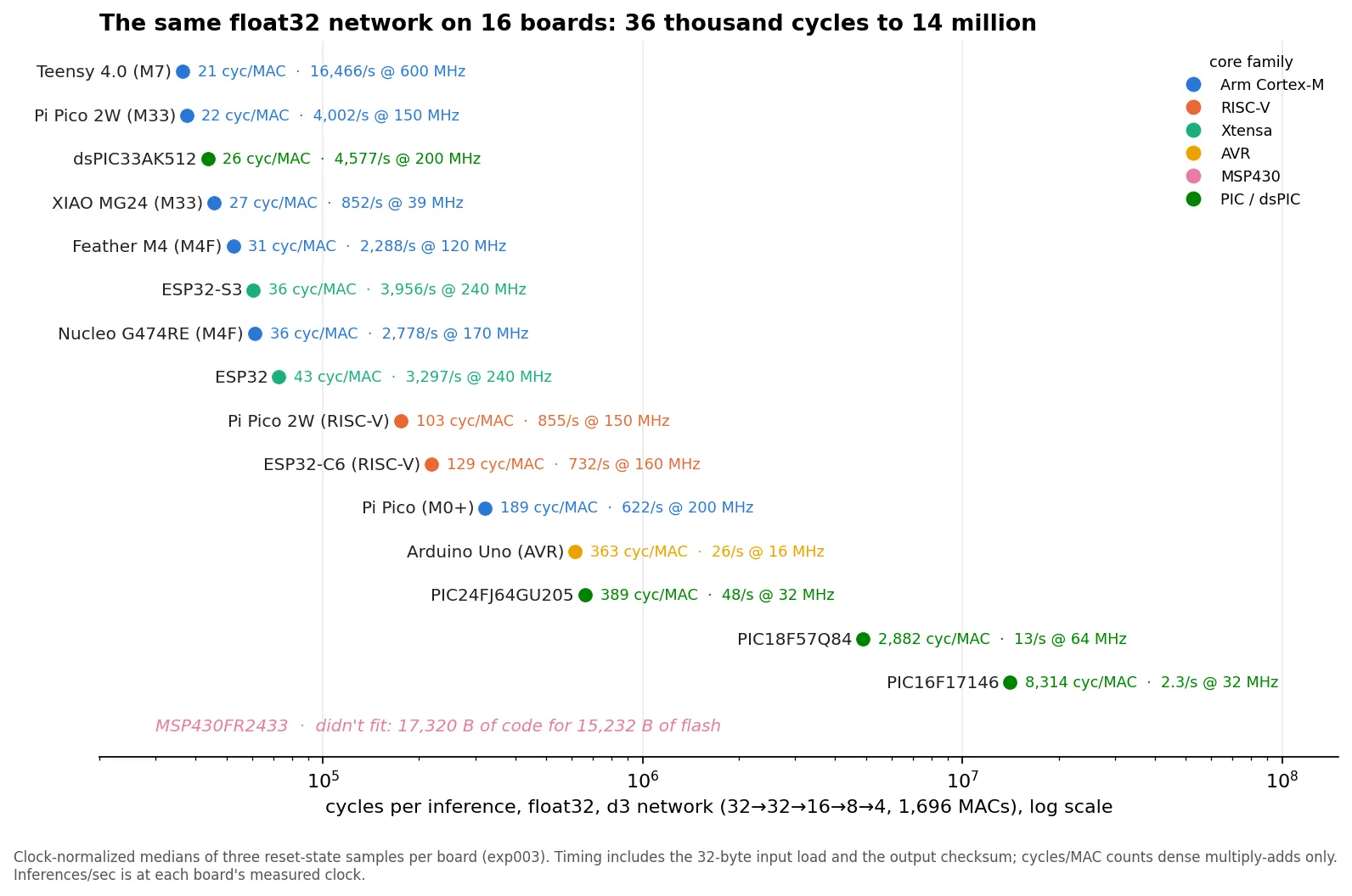
| Board | Clock | Cycles / inference | Cycles / MAC | Inferences / sec |
|---|---|---|---|---|
| Teensy 4.0 (M7) | 600 MHz | 36,440 | 21 | 16,466 |
| Pi Pico 2W (M33) | 150 MHz | 37,485 | 22 | 4,002 |
| dsPIC33AK512 | 200 MHz | 43,700 | 26 | 4,577 |
| XIAO MG24 (M33) | 39 MHz | 45,778 | 27 | 852 |
| Feather M4 (M4F) | 120 MHz | 52,438 | 31 | 2,288 |
| ESP32-S3 | 240 MHz | 60,668 | 36 | 3,956 |
| Nucleo G474RE (M4F) | 170 MHz | 61,196 | 36 | 2,778 |
| ESP32 | 240 MHz | 72,785 | 43 | 3,297 |
| Pi Pico 2W (RISC-V) | 150 MHz | 175,355 | 103 | 855 |
| ESP32-C6 (RISC-V) | 160 MHz | 218,590 | 129 | 732 |
| Pi Pico (M0+) | 200 MHz | 321,386 | 189 | 622 |
| Arduino Uno (AVR) | 16 MHz | 615,721 | 363 | 26 |
| PIC24FJ64GU205 | 32 MHz | 660,352 | 389 | 48 |
| PIC18F57Q84 | 64 MHz | 4,887,923 | 2,882 | 13 |
| PIC16F17146 | 32 MHz | 14,100,118 | 8,314 | 2.3 |
| MSP430FR2433 | 16 MHz | didn't fit | — | — |
Three things to take from that table.
Anything with a hardware FPU does this in 20 to 45 cycles per multiply-add. The Cortex-M4F, M7, M33, the dsPIC33A, and the Xtensa cores all land in the same band. At those rates the deepest network runs thousands of times a second, and for a sensor you check once a second it's a rounding error in your power budget.
No FPU costs you 4 to 10x, not 100x. The Cortex-M0+ in the original Pico, the RISC-V cores, the Uno's AVR, and the PIC24 all emulate float in software and land between 100 and 400 cycles per MAC. The Uno runs the deepest network 26 times a second. Slow, but a long way from "can't."
The 8-bit PICs are a different regime. 2,900 cycles per MAC on the PIC18 and 8,300 on the PIC16. That's the price of software float on a core with an 8-bit accumulator and a handful of registers. The PIC16 does 2.3 inferences per second. If your product decides something every few seconds, that's still enough. If it needs to be faster, keep reading.
Where float32 hits the wall
The network didn't run on the MSP430FR2433. Not because it was slow. The compiled float32 firmware came out to 17,320 bytes and the part has 15,232 bytes of program memory. 2,088 bytes over.
The PIC16 was closer than it looks, too: the float32 build used 99.9% of its program memory. One more feature in that firmware and it's out of flash. Honestly, in production you'd probably want to optimize flash use down or select a slightly larger part.
So the real boundary for a neural network on a small part isn't "does this chip do NN." The arithmetic works everywhere, it's just a loop. The boundary is three numbers you can check before writing any code:
- Product Decision Time. In your product, how long you have to make your decision after capturing your last sensor sample. For our microwave example, if it takes us 10 seconds to read sensors and then 3 seconds to decide how long to run, then even the slowest of the tested microcontrollers would complete the decision in time.
- Count your MACs. Cost scaled with multiply-adds across the whole fleet. A 1,696-MAC network costs 1,696 times whatever your core charges per MAC. This sets your time limits.
- Budget cycles per MAC by class. From the table: about 20 to 45 with an FPU, 100 to 400 with software float on a 16- or 32-bit core, 3,000 to 8,000 on an 8-bit PIC. MACs × cycles/MAC ÷ clock gives you decisions per second before you've written a line.
And then check flash. The weights alone are 7 KB in float, and the soft-float library on a part without an FPU adds a few more. On a 16 KB part that's the whole budget. Those weights are the lines in the diagrams above.
For RAM, the minimum is a pair of buffers as wide as the widest layer: two times 32 floats, 256 bytes here. There are ways to optimize these RAM and flash baselines, but it's important to understand the baselines when designing your models.
Next time: the same network, same boards, with the weights stored as 8-bit and 4-bit integers instead of floats. It fits on the MSP430. It gets faster on every single board, including the ones with FPUs. And it keeps, or in one case improves, the accuracy. That's the part people don't believe.
If you've got a model and a part and you're not sure they fit, send me the topology and the chip. I'll tell you what my numbers say, and I'm curious what you're building.
Every board in this article has a page at /fleet, and the methodology page spells out what these numbers can and can't support.
All product names and trademarks are the property of their respective owners.